Engineering Design Using Excel Worksheet

Eugene Washington, PE

 

Course Outline

1. Advantages of using EXCEL worksheets for design problems.
2. Getting started with the tool bars and formatting.
3. Excel available math function.
4. Editing commands.
5. Calculating commands.
6. Design example and discussion.
7. Protecting the worksheet.

Learning Objectives

The Engineering Design Using Excel Worksheet course is written to introduce the reader to the many advantages of computer design procedures. The goal of this course is to show the reader that computer design is easily accomplished and uses the same methods as manual computations.

At the conclusion of this course, the student will learn:

Course Introduction

So far the author has not found an engineering problem that could be better solved by hand than by using a computer. In fact, I have written programs in Excel such as a solution for soil friction circle that is so complex that few engineers even attempt to solve it by hand. These problems can take days or even weeks to find a single solution by hand and the opportunity for error is great. These same problems are solved in seconds with an Excel program and are errorless once tested and proven.

The author is not a computer Guru, so any engineer can use the Excel to effectively and efficiently create programs. The procedure is only a modification of the traditional hand written method of calculations. No special knowledge of computer programming is needed. The equations are solved exactly the same way in the computer. The computer only makes it easier by doing the calculations and keeping a record for reuse. One has only to become familiar with the Excel functions, many of which are similar to Microsoft Word.

The author performs about 95% of all engineering calculations in Excel worksheets. Workbooks are used as a filing system so all related design programs are kept together. For instance, the Excel Shoring workbook holds all the trench shoring and cofferdam design configurations. These Excel design programs have several advantages over conventional hand calculations:

A] Quickness. The programs solve in minutes that can take days by hand.

B] Accuracy. When the computer performs the calculations the chance for error is small.

C] Flexibility. These programs can easily be modified to suit the circumstances.

D] Refinement. The speed of the programs allows the designer to explore various options quickly.

E] Response. The programs allow quick solutions for field changes or unanticipated conditions.

F] Comprehensive. The programs can be made to design complete solutions and all critical components.

G] Evolution. The program can be easily expanded to include additional complexities.

H] Correction. If an error is found, it can be quickly corrected and the following calculations are automatically corrected.

I] Resources. Excel contains a comprehensive menu of math, trig, logic and statistical functions.

J] Power. Excel can perform millions of calculations per second.

K] Reuse. Once a program is written it can be reused any number of times very quickly.  

The Excel programming format is extremely powerful because its menu of math functions and the ability to sketch to illustrate the geometry being calculated. It is assumed that the reader has some computer skills, so we will proceed with the tutorial of how to design with an Excel worksheet program.  The Author explains the procedures based on the use of Excel 98.  Other versions may have a slightly different organization of the commands.

Getting Started

When an Excel workbook is first opened the screen will show a menu bar at the top of the screen. These listing are:

                               File Edit View Insert Format Tools Data Window Help

Each of these functions can be addressed from the keyboard or by clicking on them with the mouse. The first thing to do is to save the workbook with an appropriate title to describe the program. That way if you loose power or something goes wrong, you won’t loose everything you have done. Setting the automatic save prompt to every hour or so is a good precaution. Enter File, Save As and give the program any name you wish. The keyboard entry to the menu is press Alt key and the underlined letter for the menu selection. A submenu will display.

Numbers at the top of the work screen can designate the columns, but it is more difficult to write, change and debug your programming. The numbers can be changed to letters by entering Tools. Then open Options. Go into the General folder. In the top left corner under settings is a small box, which is labeled as R1C1 reference style. It will have a check mark in the box, click on the box to remove the check mark, then click OK or press the Enter key. This will now show letter headings for the columns.

Turn on the Num Lock key above the number pad. That will allow the number and formula commands to be entered more quickly. The number pad can even be used as a calculator in a cell. Select a cell and first enter =, + or -. Follow that entry with a number, then a function, then a number, etc, ending with a number. Press enter or move the cursor to another cell and the result of the calculation will be displayed. The computer will prompt if a syntax error was made and ask for a fix. If you let the computer make the fix, be sure the fix is what you want done.

The next step is to get the tool bars showing on the screen that will be commonly used to create a program. It is suggested that the Formula Tool Bar and Status Tool Bar on displayed on the screen. These tools are displayed on the screen by entering View and clicking on the tool text. It is also helpful to display the following tool bars: Standard, Formatting and Drawing. This is done be entering View, Tool bars and selecting from the pop up menu. Having these tools showing on the screen will greatly ease the programming process.

The Standard tool bar displays several important icons for easy use and quick reference. The first icon on the left is used to create a new file. The next will open an existing file. The icon that looks like a floppy disc will save your work. It is recommended that you save the work every few minutes.

The next is the printer icon. The next icon, which looks like a dog-eared page with a magnifying glass, is the print preview. It is recommended that the print range, margin, etc be checked and adjusted, if necessary, before each printing. The print can be commanded from this icon so that the number of copies and selected pages are printed. The page breaks can be adjusted to keep page continuity or print just a portion of the worksheet.

The ABC icon is a spell check command. This is very helpful to correct typos and should be used before printing.

The scissors is a shortcut paste command. This allows you to move a cell content or a block of cells from one spot to another. This can also be done with the mouse.

The next icon that looks like two sheets of paper is a copy command. This will duplicate the copied cells from one area to another. The next icon is the paste command, which can be used to place copied cells in several locations without repeating the copy command.

The curved arrow pointing left is an undo command, which helps recover from mistakes such as inadvertently deleting work or making a change that disrupts the calculations. The curved arrow pointing to the right is a redo command.  The undo command can erase up to about twenty steps of entering, but the redo is a one time only command, reversing the last undo command.

The formatting commands offer a wide range of options. For numbers there are several options that can be used: comma separators, set decimal places, currency, accounting currency, date, time, percent, fraction, scientific, text special and custom. The format can be set by individual cells or for the entire worksheet or any block of cells.

The next icon is the S icon is a summation function that will total a group of numbers over any selected range. The sum command can be typed into the computer as: =SUM(A1:A20). This will sum all the number within the range of cells A1 through A20. The summation cell must be outside the summation range or a circular error message will appear. The circular reference happens when two cells a linked to calculate using each other. The computer will not accept that. The formula calculation process must be linear.

The fx icon contains the entire math and other function commands available to use. There are far more functions than can be discussed here, but a select few will be described later during the formula creation commentary.

The A over Z and the Z over A are sort commands that will sort numerically or alphabetically across a selected range of cells. In the data menu is a much more comprehensive set of sort commands. Be careful with the sort function to include the entire range to be sorted. If a table has been created over several columns and only the first column is selected to sort, the other columns will not sort and the table will be out of sequence.

The icon with a capital A and shapes is the drawing icon, which can be turned on or off by clicking this icon.

The next to last box shows a percent number. Changing the percent increases or decreases the screen display size.

The presentation is made easier to read by aligning the text using the format alignment command. This will set the font anywhere in the cell, right, left, center and/or top and bottom. The reason the formatting tool bar is turned on is to be able to quickly format the text and numbers as needed. The first icon on the left shows the text font. You can have a global font or each cell can be different. Change the font by first highlighting the range of cells desired and then click on the down arrow on the right side of the font box. Scroll to the desired font and highlight with a mouse click and enter the change for the font.

The next box to the right that has a number showing is the font size. Enter the font size by clicking on the arrow to the right and select a number. The font will change in size when the selection is entered.

The next set of icons on the formatting tool bar is B, I, and U. These are useful when emphasis in needed. The B is for bold, which will make the letters dark and heavy. The I is for Italics, which will slant the text. U is for underlining. One or all of these icons can be turned on for a single letter or the entire text. This has been applied above in this text.

The next set of icons to the right is for the alignment of the text or numbers. Text will start at the left edge of the cell and numbers from the right edge. By clicking on these cells, the text or numbers can be right, center or left justified. The last box of this group will merge a block of cells. To do this, first highlight a block of cell and click on the box with "a" in it.

If you want to arrange the display in the merged cells, enter Format, then Cells. A menu will then show that the text can be moved, rotated, enlarged, etc. The merging of the cells can be turned off form this command menu.

The next set of icons to the right is some of the number editing commands available. The first is $ for currency. Next is the % for percentage. It is better to first format the cell that will have percentages and then enter the number. If you first enter the number 2 and then format for percent, the computer will enter 200%. If you format first then entered 2 the cell will show as 2%. The, icon will show the numbers with comma separators which aids in reading large numbers. The last icons will increase or decrease the decimal places displayed in a number. The $ and, icons will show the number in an accounting format, which will only right align the number in the cell. Under Format, Cells the number can be formatted for commas and currency and aligned as wished in the cell.

The next icons that look like lines in a page allow you to indent and move numbers within a cell. The left icon causes the justification to the left side. The center icon centers the display and the right icon justifies to the right.

The next box causes the cells to be lined around all four edges in any combination. A single cell or a block of cells can be out lined in this way. Highlight a series of cell and then click on the down arrow. A menu will display the types of outlines that can be used. To undo the outlining, click on the top left corner box when the cursor is in the cell and the outlining will disappear.

The next to last icon is used if the background color of a cell or the entire sheet needs to be changed. The last icon on the right is used to select different character colors. Both of these icons have a large selection of colors to chose from. Be careful to keep the background light or the characters can become hard to distinguish. Characters in light colors, such as yellow, are hard to read.

Editing Commands

There are several tricks that help correct errors or short cut the effort to create the computations. The first is the F2 key at the top of the keyboard, which is an edit function key. This allows you to enter any cell at any time to make whatever changes are needed. Usually, only a small part of the cell’s content needs to be changed. Enter the cell and press F2 this will allow any editing wished. Pressing F2 will also highlight all the cells in different colors that the formula in the cell addresses. This is a good feature that allows rapid review of the formula contents. The reason the formula tool bar is displayed is that it shows the actual cell formula contents above the worksheet screen while the cell shows just a number. Without the formula bar it is not possible to tell if a cell’s content is a pure number or the result of a formula. Editing can be done from the formula bar display showing the cell contents. Moving the cursor to the display and selecting the spot to edit does this. Any editing such as inserting, deleting or correction can be done to correct the formula. If the formula addresses an incorrect cell, highlight the incorrect cell coordinate with the cursor by click, hold and drag. Then release the mouse button and go to the correct cell and click on it and the formula will address the correct cell.

If you enter a cell and start typing, the entire previous cell contents will be deleted and replaced. Emptying a cell of contents can be accomplished in several ways. The Backspace key, delete key and the format, clear contents command from the mouse will empty a cell.

Press and hold the Ctrl key and Home key and the cursor will return to the top left corner of the worksheet. Press and hold the Ctrl key and the End key and the cursor will go to the bottom right end of your work. In a cell press the F2 key and Home and the cursor will go to the left cell margin. Press End key and the cursor will return to the right margin of the characters. The mouse can be used to move the cursor to any spot within the characters in the cell, or the left and right arrow keys will move the cursor.

If you want to move a formula to a different cell use the cut command. The cut command keeps the same cells as the previous calculation cell addressed. The copy command to another cell will keep the same spatial relationship as before the formula was moved. If the calculation cell addresses a cell two rows above it, when it is moved the formula cell will still address a cell two rows above. If you do not wish to change the addressed cells, use the cut command.

Both the cut and copy features can be combined in a formula. When creating a table it is common to have a formula cell address a single fixed factor and also a factor in the same row. Fixing the coordinate of the fixed cell and letting the other cell’s address to float with the cell location can solve this. An example is you want Cell D14 to contain the formula: =F2+B14*C14 and if you copy it down one row it will read: =F3+B15*C15, causing a calculation error. Cell F2 is a fixed reference. If the formula is written: =$F$2+B15*C15, F2 becomes a fixed spot that the formula will address no matter where it is copied to. The fast way to make this formula is to enter a cell D14 and type: =, then move the cursor to cell F2 and click. This will show: =F2. Now type in: +, click on cell B14, type in:*, click on cell C14. Then press Enter, go back to cell D14 where the formula reads: =F2+B14*C14 and highlight the F2 reference and press the F4 key, now the formula reads: =$F$2+B14*C14. Copy the formula down one row and the formula in cell D14 will read: =$F$2+B15*C15. $F2 will only fix the column reference and allow the row to float. F$2 will fix only the row and allow the column to float. The F4 key will change to the singular $ fixing by pressing more than once. Four presses of the F4 key will remove the $ signs. This is a very valuable shortcut when large tables are created.

Inserting rows and columns is accomplished with a few mouse clicks. For Instance, place the cursor over a row number and hold the left button down and highlight four rows. Then Press the right button while the cursor is inside of the highlighted area, select Insert and four new rows will appear. This same command will insert new columns or blocks of cells. Be careful of inserting or deleting cell that are not complete rows or columns, since that can cause a misalignment below the action.

Performing Calculations

Any cell in an Excel worksheet can contain text, number or formula. The cell can address any number of other cells to calculate a number. If you type a pure number in a cell it will be displayed as a number. If text is added to the number or the number is formatted as text, then the computer will interpreted as text. This will null any calculation attempted when addressing a cell containing text. #VALUE will appear in the formula cell indicating a calculation cannot be made. When this happens, the best way to start debugging is pressing the F2 key and examining the addressed cells to locate the error.

For the above reason and also to simplify the formula creation process, it is better to break a complex engineering design process into small components. A lengthy and complex formula is easy to get wrong and very difficult to fix.

There are several ways to create a formula in any cell. The calculation string must be started with: =, + or – sign. Now a formula can be started. If the minus (-) sign is used the formula will be calculated as a negative number. The calculation functions are:

Add: +

Subtract: -

Multiply: *

Divide: /

Exponent: ^

Less than: <

Greater than: >

Scientific notation: **

Decimal point: .

Left surround Bracket: (

Right surround Bracket: )

Now we can write formulas. Lets select a simple beam formula: M=PL/4, where a point load is placed at mid-span.

P = 1000 lbs

L = 15 ft

M = PL/4 = 3750 ft-lbs

M or the Moment can be generated in different ways. The answer can be generated by typing in: =1000*15/4. That will calculate the number 3750 and display it in the cell. The answer can also be calculated by addressing the data containing cells.

Assuming P of 1000 lbs is in cell D10 and L of 15 ft is in cell D11 and the formula is in Cell D12, type in D12:

=D10*D11/4. This will generate the 3750 number. Or type in cell D12: =, click on D10, type *, click on D11, type /, type 4 and press Enter. The Formula bar will show: =D10*D11/4. This will generate the number 3750. It is important to have the Formula bar showing so the process can be easily traced and corrected as you go.

Sometimes the solution will generate a number that has too many digits to display in a cell. The cell will display: #######. This can is the result of a couple of issues. The number may have too many digits right of the decimal point. Go to the Format tool bar and try decreasing those decimal point digits. Another solution is to widen the column until the number is displayed. Do this by going to the column designation and place on the right interface with next column and move the cursor until a left-right arrow shows. Then double click the mouse or hold and drag the mouse to the right to widen the column. This same technique can be used to make the column narrower. If the number still makes the column too wide, the number can be formatted in scientific notion; i.e. 30,000,000 will display as 3E+07. The scientific notation can also be generated by typing: 30**6 into a cell and the number 30 million will be generated.

Now let's display the above moment in K-ft. This is to demonstrate an important caution. If the formula is installed in a cell as: =P*L/4*1000, the 1000 becomes a multiplier so the number generated will be 3,750,000 not the 3.75 K-ft we were looking for. There are two ways to correct the problem. The first is to replace the * between the 4 and 1000 with a /. The formula will now be =P*L/4/1000 and show 3.75. The other way is to enclose the 4*1000 with brackets, so the formula will be P*L/(4*1000) and will show 3.75 k-ft.

It is recommended that the formula first be derived by hand and then typed in text in the computer and the data entries also be identified similar to the following:

P = Center Beam Load = 1,000 lbs

L = Beam Length = 15 ft

M = Beam Moment = PL/4 = 3,750 ft-lb

The descriptions are in one set of columns, the numbers and formula in a separate column, and the units in a third column range. This will help to keep track of what is being done, explain to others and make it easier to understand the program when you reenter it at a later date.

Now adding a uniform load to the same beam to complicate the calculation. The formula is Mw = WL^2/8. The length of L = 15ft applies. Enter the data to the previous calculation:

P = Center Beam Load = 1,000 lbs

W= Uniform Live Load = 100 lb/lf

L = Beam Length = 15 ft

Mp = Beam Moment = PL/4  = 3,750 ft-lb

Mw = Beam Live Moment = WL^2/8 = 2,813 ft-lb

Mt = Total Beam Moment  =Mp + Mw  = 6,563 ft-lb

This formula can be written two ways: =W*L^2/8 or = W*L*L/8. There is a point of caution, the computer will sometimes interpret an exponent function such as L^4/2 as L^2 and automatically edit the formula. This can be reedited and the computer will accept the formula or the function can be written as (L^4)/2 to prevent the problem from occurring.

The sum of moments can be done in several ways. A combined formula can be written: =PL/4+ML^2/8, or =Mp+Mw.

A summation : =SUM(Mp:Mw) can also be performed by the use of the S icon or by typing the command in and selecting the range of cells to sum by highlighting and Enter. The formulas and math functions can be written in by hand or selected from the Tool bars.

Usually it is helpful to have simple graphic display to illustrate the object and the design principle. In the drawing toolbar are lines, arrows, circles, rectangles and auto shapes. The only caution is that Excel is not designed to be a drafting program and the figures tend to be very memory intensive. Simple sketches can usually illustrate the object and principle used to calculate and design.

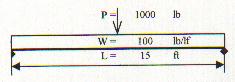
This simple sketch shows the beam with both the point and uniform loads. Note the arrows are shown with different formats. For instance, the Length arrow is formatted to be a double-ended arrow. The heavy line indicating the beam is a cell outline, and the box showing uniform load is another cell outline.

Below is an actual design program that was written in Excel and is used by the author to design cantilever sheet pile shoring. It is shown here to illustrate several useful Excel features. After the example is an explanation of the features.

The top row of this example is a descriptive name of the program so that it can be referenced easily. The date is not shown but is important. The date of the design run should be included. By entering =NOW() into a cell will display today’s date. If the date is not displayed correctly, go to Format, Cells, date or custom. The date selection is limited so usually the date is corrected in the custom view. The date can be all numbers by formatting as such: mm/dd/yy. The usual format of Jan 12, 01 is formatted as: mmm dd, yy. Many variations including time to the second can be shown. If a fixed date is wished then type into a cell: 1/12/01. That should format the cell automatically to date. Then the date can be formatted the same way as the floating date.

The date can be used as a number. The computer counts days from Jan 1,1900 so that a date in the past or future can be found by adding a number of days to any given date to find another date.

The next set of rows in the example shows the seven design criteria entries. At the right side is a table of commonly used sheet piles. Give a descriptive title with a letter symbol to each criterion and include the unit of measure. Always start a design program by entering the design criteria, preferably with numbers that will generate a known solution. That will assist in the debugging process. Each symbol is then described in a sorted table.

The next step is to write in text each formula that is to be used. The best way to list the formulas is in the same order as they are used in the calculating sequence. All the variables should be together in an area where they are easily seen. If the variables are scattered around it is easy to miss an entry and generate erroneous computations.

At this point organization is more important than presentation. Try to keep the variables and formula cells close together so that scrolling the screen is minimized. It is easier to keep track of where you are in the programming process and it will go much faster with fewer errors. Once the program is complete and calculating properly, then you can rearrange the worksheet to make a good presentation. If there is any question that a formula is improperly written, press the F2 key at any time to highlight the addressed cells and review at a glance, then edit as necessary.

Always create the formula in the same sequence as you have written it in text. For example if you wrote the formula text as Na=(Ga+Ws)X, enter the Ga, Ws and X in that order. If you sequence the data in the formula cell as Na=X(Ws+Ga) the answer will be the same. Changing the order of entry may result in a missed term and makes debugging much more difficult. Another issue is that if it becomes necessary to modify the program at a later date, it is much more difficult to understand what was previously done and how to edit it.

Start with the program formulas that are simple and use only the design criteria numbers. Once these are created, start creating the formulas that will address the ones that have already been created. That way each time a formula is completed in a cell you will see if the answer is correct or needs immediate editing. It is much easier to correct errors as you go than to debug the entire program upon completion.

Start with the simplest design solution and make sure it is working properly. Complicating features can always be introduced at a later time. The above example of a cantilever sheet pile can be made to include a water table and sloped original ground very easily.

Adjacent to the criteria numbers is a small table of sheet pile sizes and their structural properties. This is for easy reference and is used as an address for some cells. Including a table helps having to refer to a publication each time the design is performed. If such tables become large, they can be installed in separate work sheets. Addressing the table will be discussed later in this course.

One of the most useful tools is the Goal Seek command. It is very difficult to write a formula that will directly produce a direct solution for the depth of penetration of the pile. So we let computer do it for us. Goal seek requires three things in order to run. First a formula to process, second a target number and third a number that can be changed to allow the formula to calculate the target number. Try to write the formula so that the solution equals zero. The function found in Tools, Goal seek... The goal seek is started by first entering the cell address in the menu top box. Click on the formula cell showing: 0.00 to make the entry. Then zero (0) is typed into the middle menu box. Then click in the lower box and then click on the cell under X, ft showing: 10.73. Click Ok or press Enter and the iteration will begin. When a solution is found it will display OK, press Enter and the process is complete. Repeat the process for the M=0 goal seek. There are two possible reasons why goal seek will not find a solution. The first is the formula is wrong. The other reason is that sometimes the computer will search in the wrong direction. An easy check is to set the changeable number to something close to the right answer and run goal seek. If no solution is found then there is something wrong with the formulas. Goal seek is a powerful tool to help solve complex formulas that are difficult to reduce and problems that are indeterminate that can be solved only by iteration.

Below the pile cell is the text PZ35 in bold print. This cell triggers the VLOOKUP function. This function automatically brings the selected sheet pile Section Modulus and Moment of Inertia to their criteria cells. Clicking on the fx icon can enter this and selecting Lookup & Reference, select VLOOKUP and click OK. This will bring up the action necessary to import information to a cell. Move the cursor to the Sx variable cell, which now shows 48.5. Enter fx, Lookup & Reference, VLOOKUP, OK. The Lookup value is the cell showing PZ35, click on that cell. Then Table array is the range of cells inside the table showing pile type, pile Sx and pile Ix. Enter this range by highlighting the 3-cell wide by 4-cell high table with the mouse. Then click on the Col_index_num. Enter 2 as the 2^nd column for the Sx data. Repeat the command in the Ix cell except the Col_index_num is 3 for the 3^rd column in for the Ix data.

In a few places OK is displayed. This is to show that a successful solution has been achieved. If the solution does not meet the minimum design criteria, then NO GOOD will be shown. This warning feature is generated by an "if" logic statement. This is written as such: =IF(Criteria >Calc,"OK","NO GOOD"). This is a good way to show if the critical design criteria are being met or exceeded. The Criteria cell value is compared to the calculation and if the minimum criteria are exceeded, then OK is shown, if not then NO GOOD is shown. This is also found in the fx in the logic functions.

Excel has a number of trigonometry functions in fx. The main caution is that the trig functions read the angle values in radians. Notice that the Af = friction angle is shown as 30 degrees. Below is the conversion of Af from degrees to radians. This conversion can be done directly or in steps. In steps a conversion goes from 30 degrees to =RADIANS(30), which is shown as 0.52, then another cell is used to calculate a trig function, such as sine that is written as =SIN(0.52). It can also be written as =SIN(RADIANS(30)). Generally it is recommended to use the two-step approach, especially if several equations use the same angle.

Notice that all the load elements are calculated separately. Then a check that loads and reactions are equal is made to show the calculations are being done properly. This is shown as N+P+Q-R=0, check. Under is 0.00 and OK. If the loads did not balance, NO GOOD would appear notifying you that something is wrong.

The calculations are followed by a pair of simple sketches to illustrate the load distribution and the method of calculation. Note that the Math Model projects the R passive reaction to the toe of the sheet pile and projects the Q toe reaction to intersect the R projection. This method of calculation eliminates an unknown. Without this modeling technique the height of Q and the height of the intersection of the R and Q must be determined. The model now only needs to calculate the height of the upper P and Q intersection, which designated Y. This type of modeling allows for an easy and exact solution for this problem. To solve this problem without this model is either extremely complex or must be approximated.

A macro can be useful. It can be used to run the goal seek calculations with a touch of two keys. Go to Tools, Macro and click on Record New Macro. This will ask for a description and a key letter such as C. Then record the macro for both goal seeks just the same way as manually. When done be sure to stop the macro recording. This is found in Tools, Macro. Now the goal seek commands will be performed by pressing and holding the Ctrl key and pressing the C key. The main concern here is that macros are global. They will try to run in all the workbook worksheets, so be selective as to where they are applied.

One more procedure is recommended. That is protecting the work from accidental corruption. If a formula cell is accidentally entered, the entire formula can be altered or deleted. If the corruption of the cell is noticed soon enough, an undo command will restore the formula. But if the sheet is saved the formula can be lost. The sheet can be protected in a way that will allow it to be used without unprotecting it every time it is used. First, highlight the entire sheet by clicking at the top left intersection between the column and rows. Then enter Format and select Sheet, click on the Lock box to install a check mark. Click OK and exit. This locks all cells. Go back to Format and select cells. Now highlight the seven (7) input data cells and click on the Lock box and remove the check. Click on OK and exit. Now go to Tools and Protection, select protect sheet. A password is optional. If a password is used keep it simple and easy to remember. Now the only place an entry can be made is in those seven data cells.

Conclusion

This course has demonstrated how Excel computer design can be very productive. Once the program is created the program will always be available for reuse. Once proficiency is obtained, it is often faster to generate a program than to solve the same problem by hand. High accuracy and rapid solutions are obtained. The author supports field construction efforts. It is common to have an unanticipated condition suddenly crop up, and an answer is needed now!  Programs such as the above example often allow the Author to design a solution during the phone call for help. The computer is often the tool that minimizes project delays and standby costs, which can easily be several thousand dollars per hour.

Quiz

Once you finish studying the above course content, you need to take a quiz to obtain the PDH credits.

---

DISCLAIMER: The materials contained in the online course are not intended as a representation or warranty on the part of PDHonline.com or any other person/organization named herein. The materials are for general information only. They are not a substitute for competent professional advice. Application of this information to a specific project should be reviewed by a registered professional engineer. Anyone making use of the information set forth herein does so at their own risk and assumes any and all resulting liability arising therefrom.

---